I tried to recreate the Pluribus intro scene from scratch in Python with Matplotlib. Here is what it looks like:
Recently I watched a TV show produced by Apple TV called Pluribus which I really into because: 1) the key idea of “Joining” is very similar to Human Instrumentality Project from EVA, which I find very compelling; 2) I feel the narrative actually talks about relationship between humans and AI, something I have think deeply <(“)
Besides the story, I was particularly like the intro sequence. It’s minimal yet eye-catching, which is exactly my taste. While Apple TV is known for intricate intros that hint at the story’s trajectory (such as Severance or Silo), this one is distinct. It’s actually the first one I’ve seen that I think I could recreate with code :>
Since I’d never touched a particle system before and with minimum knowledge about computer vision, I kicked things off by reading a few articles. These two resources were super helpful in breaking down the concepts:
Basically, all I needed was a bunch of dots tracking their own physical state: location, velocity, and acceleration.
class Particle:
    def __init__(self, pos: (int, int),
                 velocities: (int, int),
                 accelerations: (int, int)):
        self.pos = pos
        self.vel = velocities
        self.acc = accelerations
Using the standard physics formulas we learned in high school:
\[\begin{aligned} & \boldsymbol{x}=\boldsymbol{x}_0+\int_0^t \boldsymbol{v} d t \\ & \boldsymbol{v}=\boldsymbol{v}_0+\int_0^t \boldsymbol{a} d t \end{aligned}\]I wrote a function to update those values:
def pos_update(dot, dt):
    dot.pos = (
        dot.pos[0] + dot.vel[0] * dt,
        dot.pos[1] + dot.vel[1] * dt
        )
    dot.vel = (dot.vel[0] + dot.acc[0] * dt,
                dot.vel[1] + dot.acc[1] * dt)
If we run this update loop for every dot, we get a basic working particle system (I omitted render code but this is a good tutorial about animation using matplotlib).
Finally, I added a random force to each dot. If we assume mass ($m$) is 1, then $F=ma$, so we can just add random values directly to the acceleration:
def force_apply(p: Particle):
    p.acc = (
        p.acc[0] + random.randint(-2, 2),
        p.acc[1] + random.randint(-2, 2)
        )

def dots_update(dots, dt):
    for dot in dots:
        pos_update(dot, dt)
        force_apply(dot)
    return
Here is what that looks like after initialize dots in grid:

After watching the intro five times, I realized the dots fall into three categories that I can tackle separately:
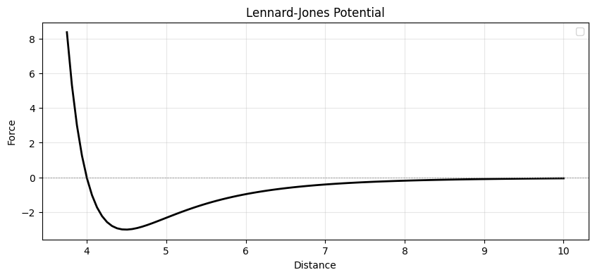
For the background dots, simple random movement doesn’t look natural. If you watch closely (make that six times now :D), you’ll see they actually interact with each other. Basically, dots push or pull one another depending on their proximity. I found that the Lennard-Jones Potential describes this behavior perfectly:
\[U_{LJ}(\vec r) = 4 \epsilon \left[ \left( \frac{\sigma}{r}\right)^{12} - \left( \frac{\sigma}{r}\right)^{6} \right],\]Essentially, when two dots are too close, they repel each other; when they are far apart (but within range), they attract. This behavior follows the curve shown below. (I learned about this from this blog).
To implement this, I simply iterate through every pair of dots to apply the force, resulting in $O(n^2)$ complexity.
def lj_force(p1, p2):
    dx = p1.pos[0] - p2.pos[0]
    dy = p1.pos[1] - p2.pos[1]
    dis = (dx**2 + dy**2) ** 0.5

    dx_dir = dx / dis
    dy_dir = dy / dis

    u = min(10, 4 * EPI * ((SIGMA/dis)**12 - (SIGMA/dis)**6))

    dx_acc = u * dx_dir / 1
    dy_acc = u * dy_dir / 1

    p1.acc = (p1.acc[0]+dx_acc, p1.acc[1]+dy_acc)
    p2.acc = (p2.acc[0]-dx_acc, p2.acc[1]-dy_acc)
Here is the result after applying the LJ potential. You can really see the complex movement emerging from the interactions between the dots.

Before adding those circle dots, I need to do a quick recap on how to define direction and distance in particle system. (You can skip if you still remember :O)
Basically given a angle $\theta \in [0, 2\pi)$ we can get the unit vector for direction
\[\begin{aligned} & \operatorname{dir}_x=\cos (\theta) \\ & \operatorname{dir}_y=\sin (\theta) \end{aligned}\]And given two points, we can get the direction from $p_1$ to $p_2$ by:
\[\begin{aligned} d x & =x_2-x_1 \\ d y & =y_2-y_1 \\ \text { distance } & =\sqrt{d x^2+d y^2} \end{aligned}\]To get the direction (unit vector), we divide the difference by the distance:
\[\begin{aligned} \operatorname{dir}_x & =d x / \text { distance } \\ \operatorname{dir}_y & =d y / \text { distance } \end{aligned}\]
Adding the circle-dots is quite easy. We just need to give them an initial speed and set their direction so they are evenly spaced around $2\pi$ (360 degrees).
def add_wave(dots):
    for i in range(WAVE_DOTS_NUM):
        angle = 2 * math.pi * i / WAVE_DOTS_NUM

        pos = (WAVE_ORIGIN[0] + math.cos(angle)*5,
            WAVE_ORIGIN[1] + math.sin(angle)*5)

        vx = WAVE_SPEED * math.cos(angle)
        vy = WAVE_SPEED * math.sin(angle)

        dots.append(Particle(pos, velocities=(vx, vy)))
The Collision Problem: However, there is a catch. Because of the Lennard-Jones force we added earlier, the background dots interact with the circle dots. As the circle expands, collisions with the background dots push the circle dots off course, distorting the shape.
The Solution: My solution was straightforward: add a mass property to the Particle class. By making the circle-dots much heavier than the background dots, they gain more inertia and aren’t easily pushed around.
I updated the physics calculation to follow Newton’s Second Law ($a=F/m$). Basically, I divide the accumulated force (acceleration) by the mass when updating the velocity:
def pos_update(dot, dt):
    dot.pos = (
        dot.pos[0] + dot.vel[0] * dt,
        dot.pos[1] + dot.vel[1] * dt
        )
    dot.vel = (
        dot.vel[0] + dot.acc[0] * dt / dot.mass,
        dot.vel[1] + dot.acc[1] * dt / dot.mass
        )
Here is a comparison of the difference (Left: without mass, Right: with mass).

After adding mass, it looks much better, doesn’t it? You can clearly see the circle dots pushing the background dots aside without losing their own formation.

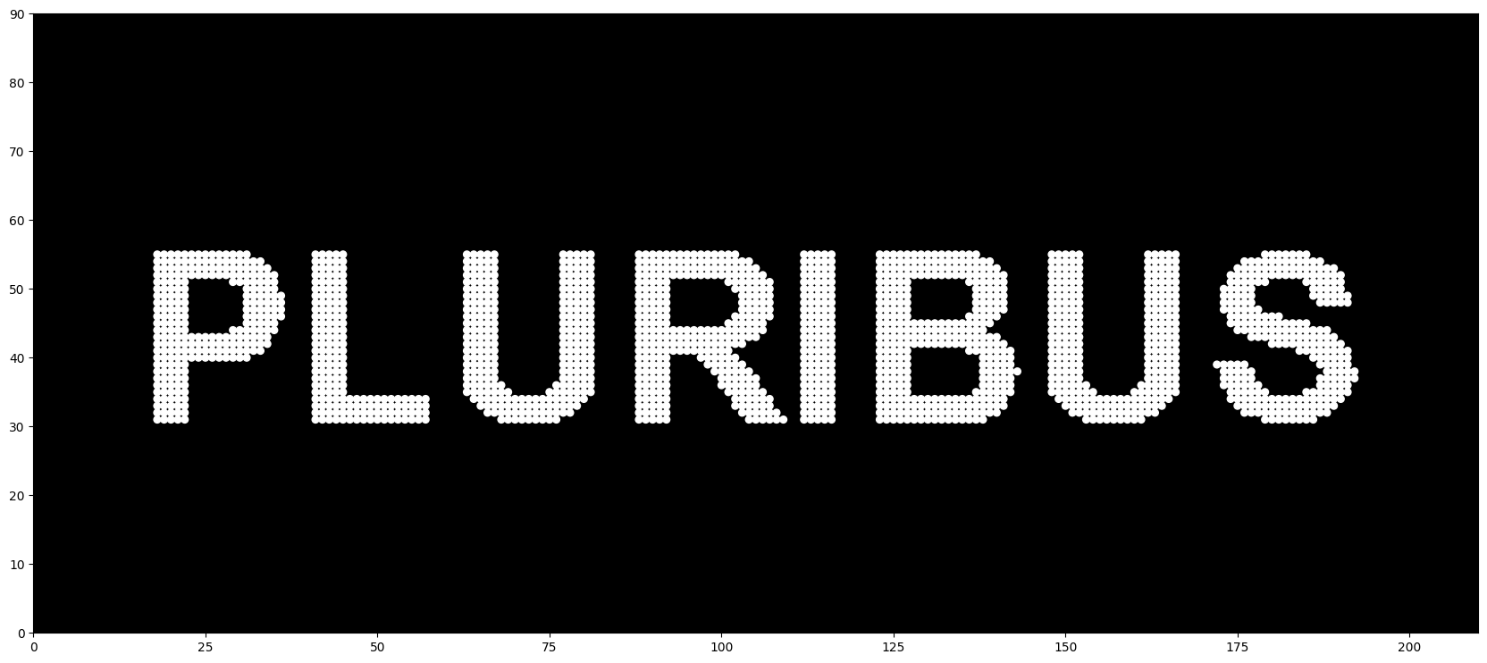
Rendering the text as dots wasn’t difficult. I simply drew the text using a font (I used Arial) and then extracted the position of every pixel from the resulting image.
def get_text_draw(text = TEXT, font_path = FONT_PATH):
    mask_img = Image.new("L", (WIDTH, LENGTH), 0)
    draw = ImageDraw.Draw(mask_img)
    font = ImageFont.truetype(font_path, 35)

    bbox = draw.textbbox((0, 0), text, font=font)
    text_w, text_h = bbox[2] - bbox[0], bbox[3] - bbox[1]
    draw.text(((WIDTH - text_w) // 2, (LENGTH - text_h) // 2 - 5), text, fill=255, font=font)
    y_coords, x_coords = np.where(np.array(mask_img)[::-1] > 128)
    return x_coords, y_coords
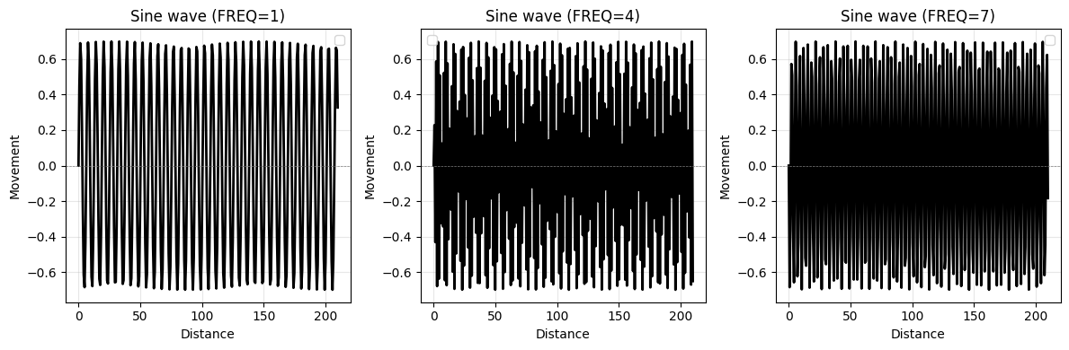
The tricky part was creating the “fingerprint” pattern. If you look closely at the original intro, it resembles a wave, though slightly irregular. For simplicity, I approximated this using a sine wave:
Basically, this pushes and pulls dots based on their distance from a center point. By adjusting the frequency, we can create different ring patterns. Following shows the effects when $freq = {1,4,7}$.
def set_fingerprint(x, y, freq = RADIAL_FREQ, strengh = RADIAL_STRENGTH):
    dx = x_coords - RADIAL_ORIGIN[0]
    dy = y_coords - RADIAL_ORIGIN[1]

    dist = np.sqrt(dx**2 + dy**2)
    angle = np.arctan2(dy, dx)

    push = np.sin(dist * freq) * strengh

    x_new = x_coords + (np.cos(angle) * push)
    y_new = y_coords + (np.sin(angle) * push)
    return x_new, y_new
Here is the result when applying the sine wave to the text, originating from point $P(25,42)$.
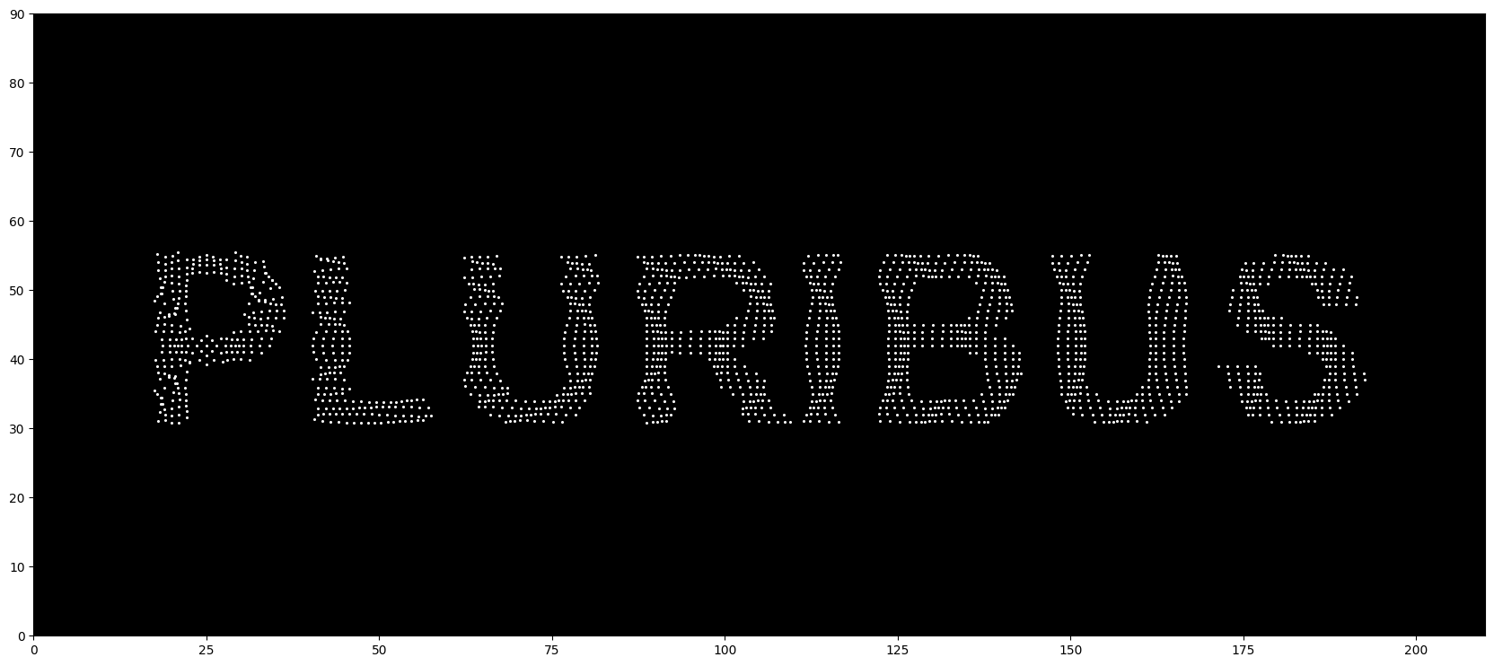
It actually took me a while to find the perfect parameters for the wave. I tested various combinations and eventually picked the one I found most satisfying. ^_^

By combining everything, we get our first version of the intro scene! 8)
Let’s pause for a moment. Currently, rendering just 60 frames takes about 6 minutes. I feel like I’m wasting my life waiting for it :( It is definitely time for some optimization.
As mentioned earlier, the main bottleneck is the physical interaction calculation, which has a complexity of $O(n^2)$. With the addition of text-dots and the continuously spawning circle-dots, the count easily hits $10^3$, meaning we are doing $10^6$ distance checks per frame.
\[size = 3 \times \sigma\] \[bin = \lfloor x / size \rfloor + numx \times \lfloor y / size \rfloor\]My solution is using bin hashing to split space into bins and only calculate the lj-force between neighbor bins. The insight is from equation from Section~3, we see that the potential becomes almost 0 when $dis \geq 3\sigma$ they are too faraway.
I created a hash map to track which bin every dot belongs to:
def _bin_coords(pos):
    return int(pos[0]) // BIN_SIZE, int(pos[1]) // BIN_SIZE

def _build_bins(dots):
    bins = {}
    for idx, p in enumerate(dots):
        bx, by = _bin_coords(p.pos)
        if 0 <= bx < BIN_XNUM and 0 <= by < BIN_YNUM:
            bins.setdefault((bx, by), []).append(idx)
    return bins
With this change, we achieved a 5x speedup, dropping the render time from 6m 10s to 1m 06s.
(I suspect there is an even more efficient way using a tree structure (something like binary-indexed tree) dynamically maintain positions and reduce complexity to $O(nlogn)$, since I’ve been doing some LeetCode lately. But this grid method is good enough for now.)
The other optimization involves controlling the lifecycle of the dots. Since the circle-dots eventually fly off-screen (“out of bounds”), we don’t need to calculate them anymore. I added a check to prune them periodically. This significantly reduced memory usage, which was previously spiking to 10GB.
def prune_dots(dots, circles, margin=50):
    alive_dots = []
    alive_circles = []

    for dot, circle in zip(dots, circles):
        x, y = dot.pos
        if -margin < x < WIDTH + margin and -margin < y < LENGTH + margin:
            alive_dots.append(dot)
            alive_circles.append(circle)
        else:
            circle.remove()

    dots[:] = alive_dots
    circles[:] = alive_circles
I’m pretty sure using a Memory Pool (with a linked list + hash map) would allow for O(1) insertion and deletion, but that’s a bit overkill for this :/
Next, let’s do some polishing on the visuals.
The first issue was that the text tended to “blur” or lose its shape over time. This happens because the dots are packed too closely, causing the Lennard-Jones potential to push them apart and we loss the finger print texture (that we thought for a long time).
My solution was straightforward: add an Anchor Force. This acts like a spring that drags the particle back to its original position if it drifts too far. I also added some damping (friction) to stop them from oscillating forever.
def anchor_force(p):
    dx = p.anchor[0] - p.pos[0]
    dy = p.anchor[1] - p.pos[1]
    dis = (dx**2 + dy**2) ** 0.5
    dx_dir = dx / dis
    dy_dir = dy / dis

    f = dis * ANCHOR_STRENGH

    damping_fx = -p.vel[0] * DAMPING
    damping_fy = -p.vel[1] * DAMPING

    p.acc = (
        p.acc[0] + (f * dx_dir + damping_fx) * random.randrange(5, 10) / 10,
        p.acc[1] + (f * dy_dir + damping_fy) * random.randrange(5, 10) / 10
        )
Another improvement was giving the background dots a “breathing” effect, where their size pulses rhythmically. To achieve this, I added a phase property to each particle and updated it over time using a sine wave.
Finally, to keep the background dots from flying off-screen, I implemented a screen warping. If a dot goes off the right edge, it reappears on the left.
def pos_update(dot, dt):
    dot.pos = (
        dot.pos[0] + dot.vel[0] * dt,
        dot.pos[1] + dot.vel[1] * dt
    )
    dot.vel = (
        dot.vel[0] + dot.acc[0] * dt / dot.mass,
        dot.vel[1] + dot.acc[1] * dt / dot.mass
    )
    dot.acc = (0, 0)

    dot.phase = (dot.phase + PHASE_INCREMENT) % (2 * math.pi)
    sine_wave = (math.sin(dot.phase) + 1) / 2

    if dot.type == 0:
        ## Keep background dots
        dot.vel = (dot.vel[0] * DECAY_RATIO, dot.vel[1] * DECAY_RATIO)
        dot.pos = (dot.pos[0] % WIDTH, dot.pos[1] % LENGTH)
        ## Change their size periodically
        dot.radius = 0.5 * (0.4 + 0.6 * sine_wave)
    else:
        dot.radius = 0.5 * (0.9 + 0.1 * sine_wave)
Here is the illustration:
Of cause you can also change the text to whatever you want:
This was my first attempt at writing a particle system. My original plan was to finish by the series finale (Christmas), but I overestimated how much energy and focus I would have while traveling. It honestly took me a while to wrap my head around how it works and how to implement it.
In contrast, I’ve seen many people use Gemini to generate fancy, interactive 3D particle systems for the web. Compared to those, my work might seem simple or even “ugly.” But for me, the experience of building this from scratch was far more enjoyable, even if it wasn’t the most efficient way. In the end, I think that feeling is also what Pluribus is talking about. :V
skewcy@gmail.com