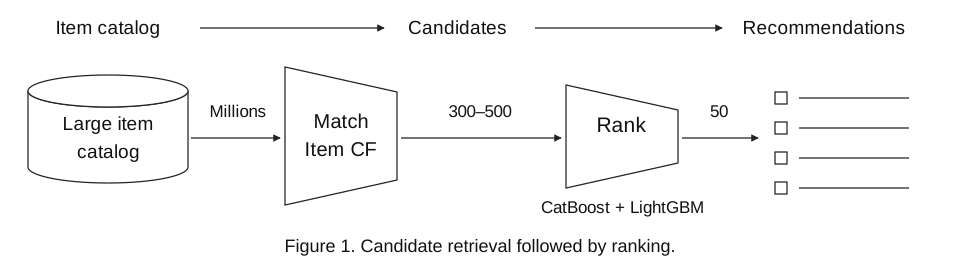
Our team, QDU, won the CIKM 2019 challenge on efficient user interest retrieval. The task was to recommend items from a huge shopping catalog, with a strict time limit and a fixed amount of memory. Our solution used Item CF for retrieval, followed by CatBoost and LightGBM for ranking.
The models were familiar. The interesting part was figuring out what to feed them, and making the whole thing run in time. :)
I worked on this with Zhuoran Zhang and Shunyao Wu. The code and team presentation are available on GitHub. This post focuses on our second-round solution; the repository also contains our qualification code.
Imagine a catalog with tens of millions of items. For each user, we need to find 50 items they may want next. Scoring every item with a large model would be too expensive, so we split the work into two steps:
The second round asked us to process about 60,000 users within one hour, in a container with 8 CPU cores, 60 GB of RAM, and a P100 GPU. Per-user retrieval also had to be sublinear in the catalog size. These were online limits; they did not mean every offline training step fit in the same container.
We had 16 days of behavior logs and needed to predict interest on day 17. The data included:
The evaluation changed between rounds. In qualification, the score combined Recall@50 and Novel-Recall@50, with novelty defined at the category level. In the second round, the recommendations had to exclude items the user had already interacted with, but could come from familiar categories.
For a user $u$, let $P_u$ be our 50 recommendations, $G_u$ the next-day ground truth, and $H_u$ the historical items. The second-round recall was:
\[\operatorname{Recall@50}(u) = \frac{|P_u \cap (G_u \setminus H_u)|} {|G_u \setminus H_u|}.\]The released evaluation code averages this over users present in its history and prediction dictionaries who have at least one eligible new item. A model trained for the qualification metric was therefore not automatically a good fit for the second round. We had to look at the data again.
For exploration, we treated days 1–14 as history and day 15 as the future. This gave us a simple question: which parts of a user’s past helped explain what they did next?
An obvious first choice was to assign behavior weights of 1, 2, 3, and 4 to page views, favorites, cart additions, and purchases. That sounds reasonable: buying something should show more interest than looking at it.
But interest in what, and for how long?
The original plot compared future activity in categories associated with different past behaviors. Categories a user had browsed still attracted activity. Categories they had already bought from showed much less. A purchase could mean that a need had been met, rather than that another purchase was coming.
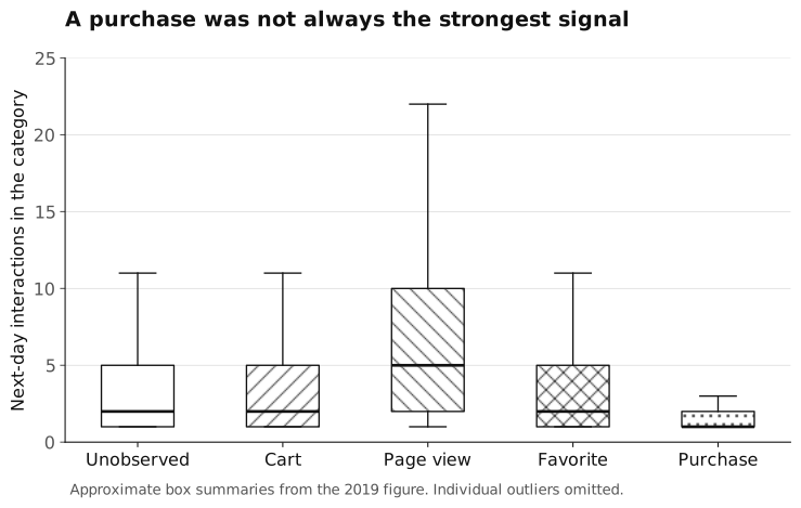
We lowered the purchase weight from 4 to 1. The resulting weights were:
\[w_{\mathrm{pv}}=1,\qquad w_{\mathrm{fav}}=2,\qquad w_{\mathrm{cart}}=3,\qquad w_{\mathrm{buy}}=1.\]This was a useful choice for this dataset, not a general rule about shopping. We could have tuned the four weights further, but ran out of time.
Next, we took the items that appeared in future behavior and counted their earlier interactions on each history day. The closer a day was to the prediction date, the more activity it contained.
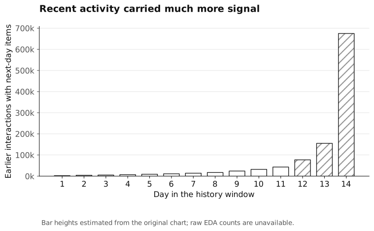
We used a simple recency weight. In the original write-up, the idea was:
\[T_{u,i} =1-\frac{D_{\max}-D_{u,i}+1}{D_{\max}-D_{\min}+1}, \qquad R_{u,i}=T_{u,i}V_{u,i},\]where $D_{u,i}$ is the interaction time and $V_{u,i}$ is its behavior weight. Recent interactions receive larger scores.
There is a small implementation detail here. The released online script uses fractional days, a $+2$ offset, and takes the maximum after weighting each event. More precisely, for an event $e$:
\[\begin{aligned} d_e &= \operatorname{day}(e)+\frac{\operatorname{hour}(e)}{24},\\ r_e &= w_{b_e}\left(1-\frac{D_{\max}-d_e+2}{D_{\max}-D_{\min}+2}\right),\\ R_{u,i} &= \max_{e:\,(u_e,i_e)=(u,i)} r_e. \end{aligned}\]Here $D_{\min}$ and $D_{\max}$ are the minimum and maximum integer days in the loaded history. The code then normalizes each user’s item weights by their sum. The idea is still simple: recent, relevant activity should count more.
Users often returned to categories they already knew. The same pattern was weaker for shops. That suggested we should keep category and shop features separate, instead of treating every kind of overlap as the same signal.
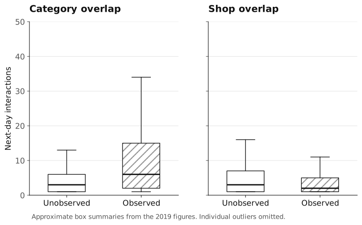
These checks were small, but they changed the design. They gave us a reason to choose a feature or a weight, rather than adding one because it appeared in someone else’s solution.
Item-based collaborative filtering, or Item CF, starts with a simple idea: items visited by the same users may be related. Build an item-to-item neighbor index from historical activity, then use each user’s history to find candidates.
Let $U_i$ be the set of users who interacted with item $i$. A basic similarity is the confidence of the rule “interested in $i$ implies interested in $j$”:
\[\operatorname{sim}(i,j) =\frac{|U_i\cap U_j|}{|U_i|}.\]This is directional. A niche item may point strongly to a popular item, while that popular item points only weakly back. In general, $\operatorname{sim}(i,j)$ and $\operatorname{sim}(j,i)$ need not be equal.
Our confidence-based retrieval scored about 0.045 online.
A user who touches hundreds of items creates many co-occurring pairs. Those pairs should not all be as informative as a pair from someone with a much shorter history.
The weighted version in the original report was:
\[w_u=\frac{1}{1+\log |I_u|},\] \[\operatorname{sim}_w(i,j) =\frac{\sum_{u\in U_i\cap U_j}w_u} {\sum_{u\in U_i}w_u},\]where $I_u$ is the set of items user $u$ interacted with. Setting every $w_u$ to 1 recovers the confidence formula. With the weighted retrieval and some additional adjustments, our online score reached about 0.053.
Code note: the public notebooks use a related, but different, formula. They count each user’s behavior rows as $c_u$, weight a co-occurring pair by $1/\log(1+c_u)$, and divide the accumulated pair count by the source item’s interaction count $c_i$. In notation:
\[A_{ij}=\sum_{u\in U_i\cap U_j}\frac{1}{\log(1+c_u)}, \qquad \widetilde{\operatorname{sim}}(i,j)=\frac{A_{ij}}{c_i}.\]The pair-count matrix $A$ is symmetric; the normalized score generally is not.
The hard part was not writing the similarity formula. It was calculating it over roughly 80 million behavior records.
We split users into groups, accumulated sparse pair counts for each group, then merged the results. Cython sped up the inner counting loop. After normalization, we kept only the top 500 neighbors for each indexed item.
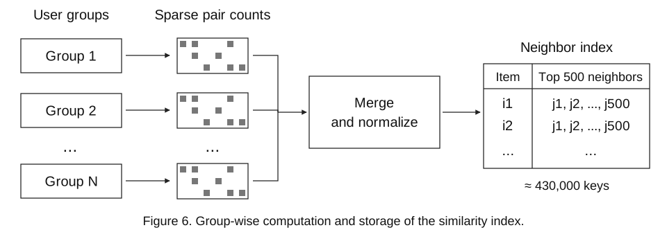
The resulting dictionary had a little over 400,000 keys, about 430,000 in our presentation. The full catalog was much larger, but we did not need to scan it for every user.
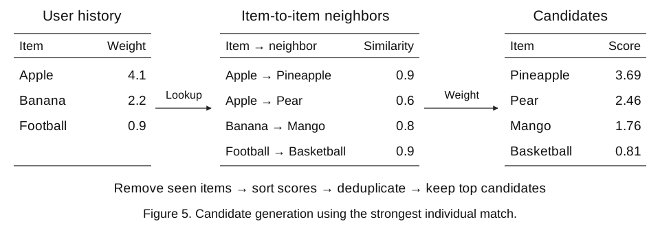
For online retrieval, we walked through the user’s history, looked up each item’s neighbors, and multiplied the neighbor scores by the user’s history weight. The released code sorts these individual matches and keeps the first occurrence of each candidate. In effect, a candidate reached through several history items keeps its strongest match; the code does not sum all those paths.
We removed previously seen items and kept a few hundred candidates. Most of the expensive work was now outside the online request. Much better. :>
There was still an offline memory cost. One candidate-generation notebook notes that it was run on a machine with 256 GB of RAM, and suggests smaller neighbor lists or batching for smaller machines. The online resource limit should not be mistaken for the memory required by the whole training pipeline.
Once retrieval reduced the catalog to 300–500 candidates, ranking became a binary classification problem: will the user interact with this candidate next?
We built the final training data from days 1–15, with labels from day 16. For prediction, we moved the history window forward to include day 16 and predicted day 17.
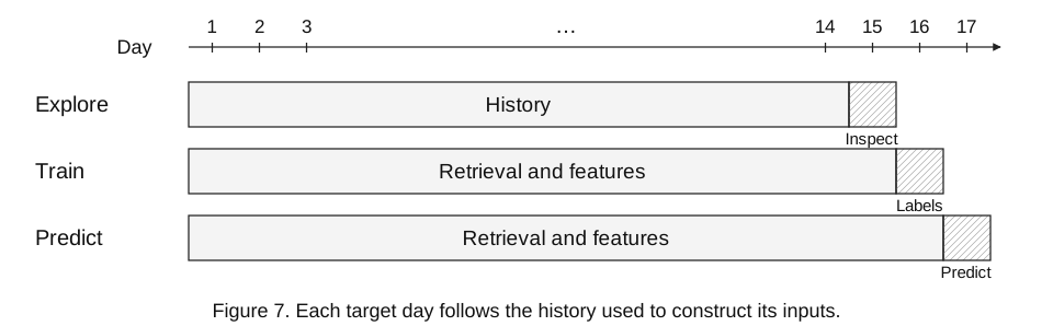
An important detail was where the positive samples came from. We did not add every future positive item to the training table. Both positive and negative samples came from the retrieval candidates.
Suppose the user later interacted with Pineapple, Pear, Bicycle, and Burger, but retrieval returned Pineapple, Pear, Mango, and Lemon. We trained on:
| Candidate | Label |
|---|---|
| Pineapple | Positive |
| Pear | Positive |
| Mango | Negative |
| Lemon | Negative |
Bicycle and Burger were missed by retrieval, so they were not ranker training samples. Those misses still hurt end-to-end recall. But inserting them into the ranker’s training data would give it examples it would not see through the same retrieval process at prediction time.
This also mattered because some retrieval-derived features were unavailable for those missing items. Keeping the training samples close to the prediction candidates worked better for us.
We built 64 features in four broad groups:
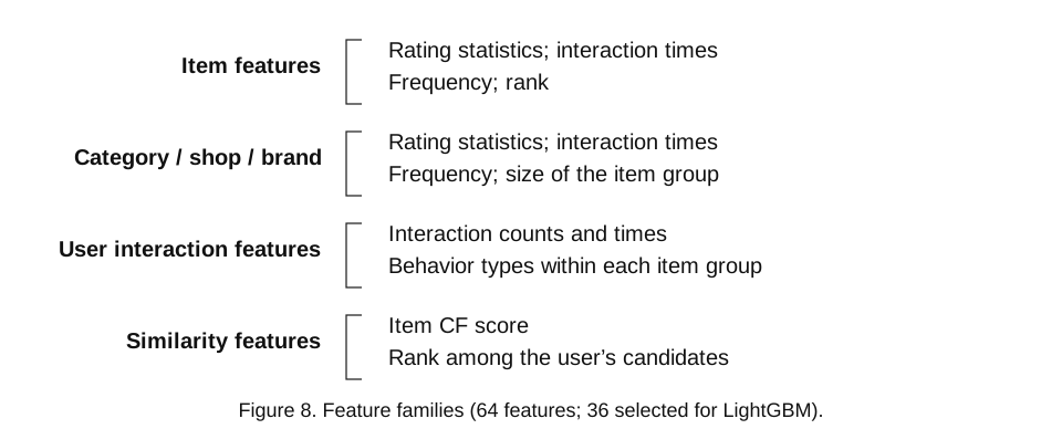
The Item CF similarity was a particularly useful feature. Retrieval had already done work to find related items, so it made sense to carry that information into ranking.
CatBoost used all 64 features and reached about 0.0616 online. LightGBM worked better with a selected set of 36. More features were not automatically better, even when the features looked useful individually.
We tried several feature-selection methods. One useful approach was the Mean Variance Index, developed in work by Hengjian Cui and collaborators. I had also packaged the method in MVTest.
The question behind it is easy to state: does a feature’s distribution change when the label changes?
Let $X$ be a continuous feature and $Y$ a categorical label. Define
\[F(x)=P(X\le x),\qquad F_r(x)=P(X\le x\mid Y=y_r),\qquad p_r=P(Y=y_r).\]The population index compares each class-conditional distribution with the overall distribution:
\[\operatorname{MV}(X\mid Y) =\sum_{r=1}^{R}p_r \int\left[F_r(x)-F(x)\right]^2\,dF(x).\]If the distributions are the same for every class with positive probability, the index is zero. Unlike a linear correlation, this comparison can also capture nonlinear dependence.
For $n$ observations, using empirical distributions gives:
\[\widehat{\operatorname{MV}}(X\mid Y) =\frac{1}{n}\sum_{r=1}^{R}\sum_{i=1}^{n} \widehat p_r\left[\widehat F_r(X_i)-\widehat F(X_i)\right]^2, \qquad T_n=n\widehat{\operatorname{MV}}(X\mid Y).\]The idea was to remove weakly associated features first, then select useful features from what remained. This gave us another view of the data alongside tree-based feature importance.
This is a marginal check, so it cannot settle every question about feature interactions. Also, my implementation at the time was slow on large datasets. A small formula does not necessarily mean a fast program. :/
We combined LightGBM and CatBoost with a harmonic mean and a geometric mean, then averaged the two results.
For positive prediction scores $a$ and $b$, the equally weighted version shown in our presentation is:
\[H(a,b)=\frac{1}{\frac{0.5}{a}+\frac{0.5}{b}}, \qquad G(a,b)=\sqrt{ab},\] \[S(a,b)=\frac{H(a,b)+G(a,b)}{2}.\]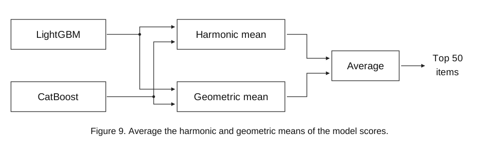
The harmonic mean is pulled down when one model gives a low score. The geometric mean is less strict, but still favors agreement. Averaging the two was a small way to balance these behaviors.
The released online script uses a slightly different geometric mean:
\[G_{\mathrm{code}}(a,b)=a^{0.48}b^{0.52},\]where $a$ is LightGBM’s score and $b$ is CatBoost’s. Its harmonic mean remains equally weighted. We then sorted candidates by the combined score and returned the top 50, with popular-item fallbacks for short lists or users without candidates.
The original post reported an online score of 0.0622 for the ensemble. Here are a few checkpoints from the write-up:
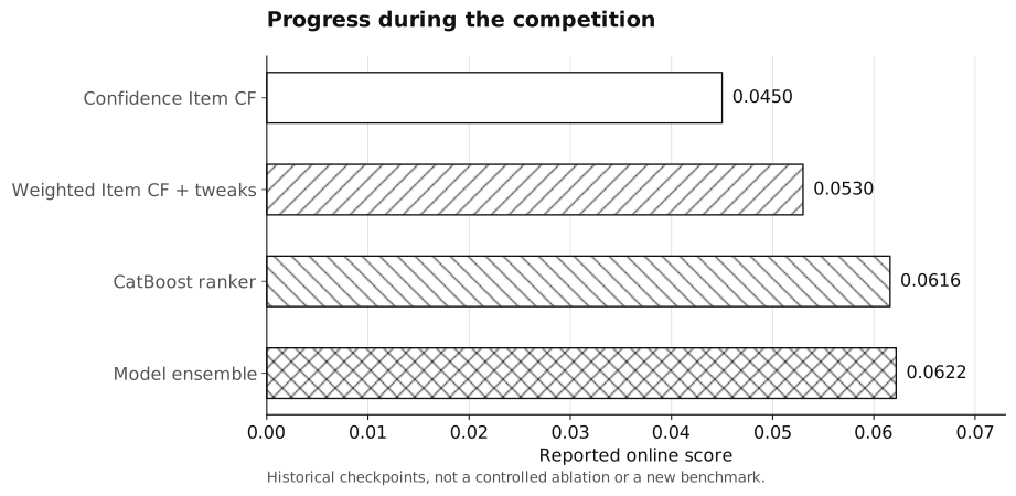
These are results from different stages of the competition, not a controlled ablation. In particular, the weighted Item CF result included other adjustments. The team slides record 0.06222 and second place on the second-round leaderboard; the repository identifies the team as the overall challenge winner. Those describe different stages of the competition.
We also explored category-based and shop-based rules, Word2Vec-style embeddings with FAISS, MinHash LSH for Item CF, and limiting the history to recent interactions.
Not all of these became part of the final pipeline. We did not finish a fair comparison of every approach, so I would not read the final choice as proof that Item CF always beats an embedding model. It was a method we could make work well within our time and resource limits.
The most useful ideas came from looking closely at the data: a purchase did not always mean more future interest; recent actions mattered more; a familiar category was different from a familiar shop. Those observations shaped the retrieval scores and the features before we spent much time on model tuning.
The engineering mattered just as much. Sparse counts, parallel work, short neighbor lists, and Cython turned a reasonable idea into a pipeline we could submit. Getting the sampling right mattered too: the ranker needed to learn from the candidates it would actually receive.
I still think ideas are more useful than recipes. Read the data, try a small change, see what happens, and read a paper when you get stuck. There is often more to gain there than from one more round of parameter tuning.
And sleep before the deadline. That part is surprisingly easy to forget. :)
skewcy@gmail.com