I joined the BDCI 2020 traffic forecasting competition and finished 12th in the semifinal round. The project started as my final project for CSE 5095, Machine Learning for Time Series Analysis, at UConn. I wanted to try a few ideas from the course on a real problem. The code and report are on GitHub.
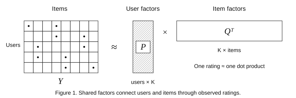
The idea I found most interesting came from recommendation systems. A user–item rating matrix has many empty cells, but users and items still share patterns. Traffic data has a similar structure: many roads, many time points, and many missing observations. Could matrix factorization make this forecasting problem easier?
It turned out to be a useful starting point. I learned a small set of road and time factors, predicted the future time factors, and used a classifier to turn them into traffic states. :)
The competition asked us to predict a road segment’s traffic state at a future time. Each query came with recent observations from the same day and observations around similar times in earlier weeks. Road attributes and upstream/downstream connections were also available.
I arranged the traffic observations as a matrix:
\[Y\in\mathbb R^{n\times T},\qquad n=15{,}584,\qquad T=31\times720=22{,}320.\]Each row is a road segment. Each column is a two-minute time slot. The matrix spans 31 days, with 720 slots per day. About 74.7% of its entries are missing.
This creates two problems. First, the road series are related: a queue on one road can affect nearby roads, and distant roads can follow similar daily patterns. Training a separate model for every road would miss these shared patterns. Second, filling all the gaps before training can introduce errors that the forecasting model then treats as real observations.
I wanted a representation that could learn from the entries we actually had, share information across roads, and stay small enough to experiment with.
In a matrix factorization recommender, a user and an item each get a short vector. Their dot product estimates the user’s rating for the item:
\[\hat Y_{u,i}=p_u^\top q_i.\]The vectors are learned together. A user with only a few ratings can still benefit from patterns learned from other users and items.
For traffic, replace users with roads and items with time slots. Let $P\in\mathbb R^{n\times K}$ contain the road factors and $Q\in\mathbb R^{T\times K}$ contain the time factors. Then
\[Y\approx PQ^\top,\qquad \hat Y_{i,t}=p_i^\top q_t.\]A usual regularized formulation is
\[\begin{aligned} \min_{P,Q}\quad &\sum_{(i,t)\in\Omega} \left(Y_{i,t}-p_i^\top q_t\right)^2\\ &+\lambda_P\lVert P\rVert_F^2 +\lambda_Q\lVert Q\rVert_F^2, \end{aligned}\]where $\Omega$ is the set of observed road–time pairs. The sum over $\Omega$ matters: a missing observation is not a traffic state of zero.
I used alternating least squares. Hold the time factors fixed and update the road factors; then hold the road factors fixed and update the time factors. Each update fits the observations associated with that road or time slot.
The notebook uses 64 factors. The full matrix has about 348 million positions, while the two factor matrices have about 2.43 million values. This is a much smaller representation, although constructing the data and intermediate arrays still takes substantial memory.
The useful part is the sharing. A time factor describes a pattern across many roads, and each road factor describes how that road participates in those patterns. Missing entries do not have to be filled with guessed labels before fitting. A road with little data can borrow information through the shared factors, though a road with no useful observations still needs a fallback.
Matrix factorization explains the observed matrix. To predict beyond it, we still need a time-series model.
The time-factor matrix gives us $K$ dense series to forecast. I kept the road factors fixed, predicted new time factors, and used their product as a first estimate of future traffic:
\[\hat Y_{\mathrm{future}}=P\hat Q_{\mathrm{future}}^\top.\]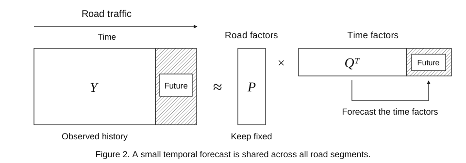
This changes the size of the forecasting problem. Instead of directly forecasting 15,584 sparse road series, the temporal model works with 64 dense factor coordinates. It can focus on how the shared patterns change over time.
Of course, the compression loses information. The factors can capture common patterns while smoothing away details that matter for a particular road. That becomes important when we add the final classifier.
The data had a clear daily rhythm, with differences between days of the week. I could also see this rhythm after factorization. The following plot shows the mean of the time-factor coordinates at each time slot.
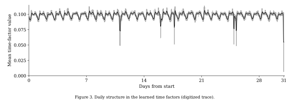
The vertical scale belongs to the learned factors; it is not a traffic speed or a congestion measurement. I used this average as a quick visual check of the representation.
For prediction, I started with a seasonal average and a weekly scale factor. Let $d$ be the day index and $s$ the time slot within a day. Write $r(d)$ for the day of the week and $w(d)$ for the week index. For each day of the week, average the time factors at the same slot:
\[\bar q_{r,s} =\frac{1}{|\mathcal D_r|} \sum_{d\in\mathcal D_r}q_{d,s},\]where $\mathcal D_r$ contains the reference days with weekday $r$. The notebook builds these profiles from the first four weeks.
The prediction then takes the form
\[\hat q_{d,s}=a_{w(d)}\,\bar q_{r(d),s}.\]Here $a_w$ adjusts the overall level for week $w$. In the notebook, this scale comes from the mean observed traffic level in the first three days of each week, normalized by the mean across those weekly estimates. The scale is shared across the factor coordinates and time slots within the week.
For example, to estimate a Thursday evening, start with the average factor vector for that Thursday slot and adjust it by the week’s scale. The method is simple, and its assumptions are easy to inspect. When forecasting, the scale also has to come from observations available before the target time.
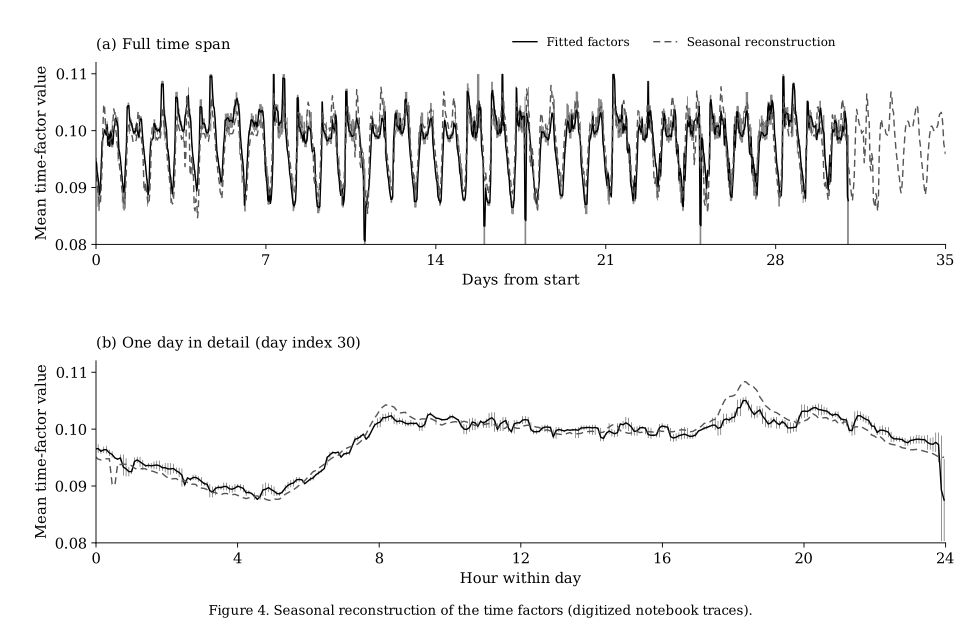
The seasonal reconstruction follows much of the broad shape. It is a useful check that the periodic structure survived factorization. It does not capture every local change, and matching the factor trace alone does not tell us how well the final traffic labels will be predicted.
A sequence-to-sequence model would be a natural next experiment. It could learn changes that a fixed weekday profile misses. I left that as future work; the solution here uses the simple seasonal model.
The factorization learns relationships from traffic observations, but the task also gives us a road network. I added three ways to group roads:
| View | How I built it | Feature |
|---|---|---|
| Road topology | Build a graph from upstream/downstream connections and run Louvain community detection. | Topology community ID. |
| Traffic similarity | Connect roads with high cosine similarity between their traffic histories and run Louvain again. | Traffic-similarity community ID. |
| Road factors | Cluster the road-factor vectors with K-means. | Factor cluster ID. |
These views answer different questions. Two roads can be physically connected without having the same traffic pattern. Two roads can have similar rush hours without being close together.
I represented each road segment as a node and each supplied connection as an edge. For community detection, I used an undirected graph with unit edge weights.
The Louvain method looks for groups with more internal connectivity than a degree-based reference model would suggest. Its modularity objective is
\[\mathcal M =\frac{1}{2m}\sum_{i,j} \left(A_{ij}-\frac{k_i k_j}{2m}\right) \mathbf 1[c_i=c_j],\]where $A$ is the adjacency matrix, $k_i=\sum_j A_{ij}$ is the weighted degree, $m=\frac12\sum_{i,j}A_{ij}$, and $c_i$ is the community assigned to road $i$.
The community ID gives the classifier a coarse description of where a road sits in the network. It is a compact feature; it does not model how congestion moves along individual directed edges.
For the traffic-similarity graph, I compared transformed traffic-history vectors $z_i$ with cosine similarity:
\[s_{ij}=\frac{z_i^\top z_j} {\lVert z_i\rVert_2\lVert z_j\rVert_2}.\]The transformation sets missing entries and the lowest encoded states to zero. This makes the graph focus on shared higher-state activity. I kept similarities above the 75th percentile of positive similarities as weighted edges, then applied Louvain to that graph.
The third view was cheaper to construct: run K-means on the 64-dimensional road factors $P$. I used 24 clusters. Together, these features describe physical connections, observed behavior, and the patterns learned by factorization.
There is one more mismatch to fix. The target is a discrete traffic state, while the dot product produces a continuous number.
If the prediction is 3.6, should the answer be state 3 or state 4? Rounding is possible, but it assumes that the numerical spacing between the state codes is meaningful. The codes do not tell us that a change from 1 to 2 has the same meaning as a change from 3 to 4.
I therefore used the factors as inputs to a multiclass CatBoost model. For road $i$ and target time $t$, the final prediction is
\[\hat y_{i,t} =f\!\left(p_i,\hat q_t, p_i^\top\hat q_t, x_{i,t},c_i\right) \in\{1,2,3,4\},\]where $x_{i,t}$ contains traffic statistics and road attributes, and $c_i$ collects the road-group features.
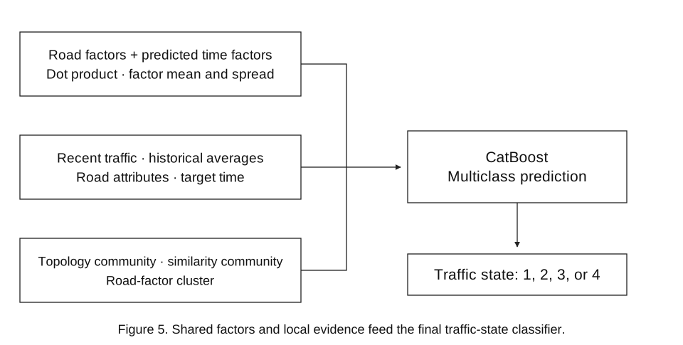
The extra features included recent speed and state observations, time until the prediction target, road attributes, and historical averages around the target slot on earlier days and weeks. I also added the mean and standard deviation of each factor vector, together with the dot-product estimate.
This lets the classifier combine a broad shared pattern with more local evidence. For example, the time factors may describe a typical evening, while recent observations tell us that one road is already unusually busy.
In my competition experiments, adding the classifier to the factor representation improved the online weighted F1 score by about 48% relative to direct factor-product prediction. Adding the traffic statistics and road relationships brought the improvement to about 96% over that same baseline. These are relative improvements, not percentage-point gains.
The final solution placed 12th in the semifinal round. Most of my limited submissions went toward comparing ideas, so there was still room to improve the feature choices and training setup.
The most useful idea was to change the representation before making the forecasting model more complicated. Matrix factorization gave me a small shared space in which a simple temporal model was already useful. The classifier then recovered some of the detail that the factorization could not preserve.
The practical side mattered too. Large intermediate arrays and repeated feature calculations made memory a real constraint. A machine with around 128 GB of RAM made these experiments much easier; otherwise, batching and waiting would have taken a large part of the time I had.
This began as a course project, and trying the methods on real data taught me more than tuning one model for a little longer would have. There are several parts I would like to revisit, especially learning the time-factor forecast and building a stronger temporal validation setup. For now, I am glad this recommendation-system idea turned into a working traffic solution. :>
Thanks to supermanwasd for providing the computing environment, and to Dongjin Song for the paper discussions in CSE 5095 that inspired this project.
The solution repository contains the five notebooks and the course report. Figure sources and redraw code are also available.
skewcy@gmail.com