I joined the Challengers team for the KDD Cup 2020 Debiasing Challenge. We finished first on the A leaderboard and sixth on the final B leaderboard. Our solution and code are on GitHub.
The task was to predict a user’s next click. The interesting part was doing this well for items that had received little exposure. A recommender could look good overall while mostly recommending the same popular items. This competition made us pay attention to the items it was missing.
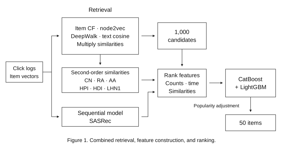
We used Item CF, graph embeddings, and text similarity to find candidates, then CatBoost and LightGBM to rank them. Most of the useful work happened around these models: how we combined similarities, how we described changing popularity, and how we built the training data. :)
The Debiasing Challenge provided five kinds of files:
| Data | What it contained |
|---|---|
| User features | User ID, age, gender, and city, with many missing values. |
| Item features | A 128-dimensional image vector and a 128-dimensional text vector for each available item. |
| Training clicks | User ID, item ID, and timestamp. |
| Test-user histories | The observed clicks of the users we needed to recommend for. |
| Query times | When to predict each test user’s next click, without revealing the item. |
Click logs arrived in phases, numbered 0 through 9. Their distributions changed over time, including a large burst of activity that looked like a promotion. Phases 0–6 were used during development; the final evaluation used phases 7–9.
We returned 50 items for each query. With one next-click target, NDCG@50 has a simple form. If the target is at position $r$, counting from 1, its contribution is
\[g(r)= \begin{cases} 1/\log_2(r+1), & 1\leq r\leq 50,\\ 0, & \text{if the target is not in the list}. \end{cases}\]The evaluation averaged this score over two sets of queries:
The full score determined eligibility: a team needed to be in the top 10%. Among eligible teams, the half score determined the final ranking. This made the tradeoff concrete. We needed to find less popular items without losing too much accuracy overall.
We first retrieved up to 1,000 candidates for each user. We then built features for each user–candidate pair and trained a binary classifier to predict the next click. The final step combined the models, applied a popularity adjustment, and returned 50 items.
The sequential model had a different job from the retrieval models. It contributed a ranking feature. The second-order graph similarities also became ranking features in our final solution.
The phase files overlapped, so we removed duplicate user–item–timestamp records when combining them. We also combined the training clicks with the observed test-user histories. Those histories were inputs to the task, not the unknown next-click answers.
For users with enough history, we made two local datasets:
At each step, the remaining history supplied retrieval and feature construction.
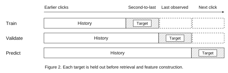
The important detail was removing held-out user–item interactions from every phase where they appeared. Deleting a label from one file was not enough if the same interaction remained in another file.
We kept separate data paths for local training, validation, and final prediction. That made it easier to use the same sequence of steps without accidentally mixing their inputs.
Item-based collaborative filtering connects items through shared user activity. We added weights for the distance between clicks, their order, user activity, and item popularity.
Here is the calculation broken into smaller pieces. For two positions $a$ and $b$ in a user’s click sequence, define
\[\begin{aligned} w_{\mathrm{pos}}(a,b) &=\max\!\left(0.5,\;0.9^{|a-b|-1}\right),\\ w_{\mathrm{time}}(u,a,b) &=\max\!\left(0.5,\;\frac{1}{1+650000\,|t_{u,a}-t_{u,b}|}\right),\\ w_{\mathrm{dir}}(a,b) &= \begin{cases} 1, & b>a,\\ 0.8, & b<a. \end{cases} \end{aligned}\]Nearby clicks receive more weight. The direction term gives a larger weight to an item that comes after the source item. The factor 650000 sets the time scale for the competition’s timestamps.
Let $n_i$ be the number of clicks on item $i$, $m_i$ the number of distinct users who clicked it, and $L_u$ the length of user $u$’s history. Let $\mathcal P_{ij}$ contain the ordered pairs of clicks on $i$ and $j$ within the same user’s history. Then
\[S_{\mathrm{CF}}(i,j)= \frac{1}{(n_i n_j)^{0.2}} \sum_{(u,a,b)\in\mathcal P_{ij}} \frac{ w_{\mathrm{dir}}(a,b)\, w_{\mathrm{pos}}(a,b)\, w_{\mathrm{time}}(u,a,b) }{ \log(1+m_i)\,\log(1+L_u) }.\]The denominator matters as much as the numerator. A very active user creates many item pairs, and a popular item appears in many histories. Without some correction, both can dominate the similarity score.
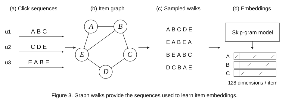
Click sequences also give us an item graph. We connected consecutive items, generated walks through the graph, and trained a Word2Vec-style model on those walks. Items that appeared in similar contexts could then have similar embeddings, even if their direct co-occurrence was weak.
We used two versions:
For DeepWalk, if $N(i)$ is the neighbor set,
\[P(j\mid i)=\frac{1}{|N(i)|}, \qquad j\in N(i).\]For node2vec, the next step also depends on the previous node. If the walk arrived at $i$ from $v$, we sample a neighbor $j$ with probability
\[P(j\mid v,i)= \frac{\alpha_{p,q}(v,j)\,e_{ij}} {\sum_{k\in N(i)}\alpha_{p,q}(v,k)\,e_{ik}},\]where $e_{ij}$ is the edge weight. The bias factor is $1/p$ for returning to $v$, 1 when the next node is connected back to $v$, and $1/q$ otherwise. We used $p=2$ and $q=0.5$, which reduced immediate returns and encouraged exploration farther from the previous node.
Both models used walks of length 20 and learned 128-dimensional item embeddings. We measured item similarity with cosine similarity. The supplied text vectors gave us another cosine similarity, based on item descriptions.
We shifted each cosine similarity from $[-1,1]$ to $[0,1]$:
\[\widetilde s(i,j)=\frac{1+\cos(\mathbf e_i,\mathbf e_j)}{2}.\]The combined item similarity was
\[S(i,j)= S_{\mathrm{CF}}(i,j)\, \widetilde s_{\mathrm{node}}(i,j)^2\, \widetilde s_{\mathrm{deep}}(i,j)\, \widetilde s_{\mathrm{text}}(i,j).\]Multiplication makes agreement useful. A pair supported by several views can stay strong, while a weak signal in one view can reduce its score. For unavailable embedding similarities, we used 0.5, the value corresponding to zero cosine similarity.
For each user, we visited the items in their history, looked up each item’s top 500 neighbors, and accumulated weighted scores for the candidates. Recent history received more weight. We removed already-clicked items and kept the top 1,000.
We also tried taking the union of separate retrieval lists. Multiplying the similarities worked better for us. My guess was that it changed which low-frequency items survived the top-$K$ cutoff. User CF was less useful: its individual recall was weak, and it overlapped heavily with Item CF.
One competition-specific trick was to use all the released click logs when building similarities. For a target phase $T$, we shifted the timestamps of phases $T+1$ through 9 to before phase 0. This kept phases 0 through $T$ at the recent end of the sequence while adding more co-occurrence evidence.
This helped more on the A leaderboard than on the final phases 7–9, where there was less data after the target phase to reuse. It may have been one reason our early ranking did not carry over to the final result.
Two items can be related through their neighbors even when they have no direct similarity edge. In the figure below, $x$ and $y$ both connect through $z_1$, $z_2$, and $z_3$.
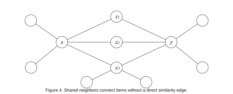
We built a sparse graph from the combined item similarities and calculated six second-order measures: Common Neighbors, Resource Allocation, Adamic–Adar, Hub Promoted Index, Hub Depressed Index, and Leicht–Holme–Newman.
Two examples show the idea. Let $W_{ij}$ be the retained edge weight and let
\[s_i=\sum_{k\in N(i)}W_{ik}\]be the node’s weighted strength. Let $\mathcal Z_{ij}$ be the intermediate items found by the neighbor search. The weighted Adamic–Adar score is
\[S_{\mathrm{AA}}(i,j)= \sum_{z\in\mathcal Z_{ij}} \frac{W_{iz}W_{zj}}{\log(1+s_z)}.\]A connection through a very well-connected item receives less weight. The Hub Promoted Index uses a different normalization:
\[S_{\mathrm{HPI}}(i,j)= \frac{\sum_{z\in\mathcal Z_{ij}}W_{iz}W_{zj}} {\min(s_i,s_j)}.\]We tried these measures in retrieval during the A stage. With less time and computing capacity before the B submission, we used them as ranking features instead. They gave the ranker information about the neighborhood around a candidate, beyond the direct match that retrieved it.
The candidate table let us turn recommendation into a binary classification problem: for this user, will this candidate be the next click?
We built features in five groups:
| Group | Examples |
|---|---|
| Similarity | Item CF, graph similarities, text and image similarities, and summaries over the user’s history. |
| Item popularity | Click counts by phase, changes between phases, and distance from the item’s peak or lowest count. |
| Time | Recent click counts, time gaps, and similarity to the user’s most recent item. |
| User–item interactions | How the candidate’s popularity compared with the popularity of items in the user’s history. |
| Sequential model | A score from a self-attentive recommendation model. |
The similarity summaries included maximum, mean, variance, and accumulated scores where appropriate. We built 23 similarity features, 18 item-click features, and 11 time features, along with the interaction and sequential-model features.
The phase-aware click features made a large difference. A count alone cannot tell us whether an item is becoming popular, fading out, or returning after a quiet period. Comparing counts across phases gave the model some of that context.
This helped us train one model across phases with different distributions. Instead of asking the model to treat every period as if it looked the same, we supplied features that described how it differed.
We also tried Self-Attentive Sequential Recommendation, or SASRec. It reads the user’s click sequence and learns which earlier items are relevant to the next prediction.
We initialized item embeddings with the 256-dimensional image-and-text vectors, scaled by $1/25$. Our prediction layer combined the sequence representation $\mathbf f_{u,t}$ with a learned user embedding $\mathbf e_u$:
\[r_{u,i,t}= (\mathbf f_{u,t}+\mathbf e_u)^\top\mathbf m_i, \qquad p_{u,i,t}=\frac{1}{1+\exp(-r_{u,i,t})},\]where $\mathbf m_i$ is the candidate item’s embedding. We passed the sigmoid score to the ranker.
The model did not work well enough as a standalone retrieval method, but its score helped the ranking model. That was a useful reminder: a model can contribute something valuable without owning the whole pipeline. :>
We used the Mean Variance Index to screen features and kept 58 for ranking. I had also implemented this method in MVTest.
The test asks whether a feature’s distribution changes with the class label. For a continuous feature $X$ and a discrete label $Y$, its population form is
\[\operatorname{MV}(X\mid Y)= \sum_c p_c\int \left[F_c(x)-F(x)\right]^2\,dF(x),\]where $F$ is the overall distribution of $X$, $F_c$ is its distribution within class $c$, and $p_c$ is that class’s probability.
This gave us a view of feature relevance that differed from tree-based importance. A feature could be useful even when its relationship with the label was not linear. I described the method in more detail in my CIKM 2019 post.
Positive samples were the retrieved candidates that matched the held-out next click. Negative samples came from the same candidate lists. We sampled five negatives per positive, so the ranker learned from the kinds of items it would actually receive at prediction time.
We made six datasets with different random samples of the negatives. Each dataset trained a CatBoost model and a LightGBM model. We then averaged the six predictions within each model family.
We also gave more training weight to low-count items, especially positive examples. This made errors on rare clicked items more expensive during training, rather than leaving all of the debiasing work to the final sort.
Let $C$ and $L$ be the averaged CatBoost and LightGBM scores. We combined a weighted harmonic mean and a weighted geometric mean:
\[\begin{aligned} H(C,L)&=\frac{10}{6/C+4/L},\\ G(C,L)&=C^{0.6}L^{0.4},\\ S(C,L)&=H(C,L)+G(C,L). \end{aligned}\]Both terms give CatBoost a weight of 0.6 and LightGBM a weight of 0.4. The harmonic mean is especially sensitive to one model assigning a low score. The geometric mean also rewards agreement, but less strongly.
The final submission allowed little room for trial and error. We kept the last adjustment simple: reduce the relative advantage of popular items.
For an item with a positive cumulative click count $n_i$ through the query phase, the multiplier was
\[b(i)=\max\!\left(0.61,\frac{1}{\log(n_i+2)}\right).\]We multiplied each model’s score by this factor before combining them. Because both ensemble terms scale linearly when their two inputs are multiplied by the same positive factor, this is equivalent to
\[S_{\mathrm{final}}(u,i)=b(i)\,S(C_{u,i},L_{u,i}).\]The floor limited how much we reduced a score. This gave a small improvement on the half score while leaving the full score roughly unchanged. We sorted the candidates by the final score and returned 50 items.
The most useful features described the data distribution itself. Popularity was changing across phases, so features about those changes mattered more than a single global count.
Carefully weighted Item CF was still a strong starting point. Graph embeddings, text vectors, and second-order similarities added different views of the same items. The challenge was deciding how to combine them, then computing them efficiently.
I also came away with more respect for the data split. Retrieval, feature generation, and ranking all need to agree about which clicks are available. Getting that right early saves a lot of confusion later.
And leave time to try an idea that does not fit the current plan. The sequential model was disappointing as a retriever and useful as a feature. We would have missed that if we had judged it only by its first result.
One final lesson: a competition with one final submission can produce a very long evening. :/
skewcy@gmail.com